Assessing Classical Test Assumptions
In classical parametric procedures we often assume normality and constant variance for the model error term. Methods of exploring these assumptions in an ANOVA/ANCOVA/MANOVA framework are discussed here. Regression diagnostics are covered under multiple linear regression.
Outliers
Since outliers can severly affect normality and homogeneity of variance, methods for detecting disparate observerations are described first.
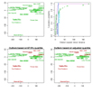
The aq.plot() function in the mvoutlier package allows you to identfy multivariate outliers by plotting the ordered squared robust Mahalanobis distances of the observations against the empirical distribution function of the MD2i. Input consists of a matrix or data frame. The function produces 4 graphs and returns a boolean vector identifying the outliers.
# Detect Outliers in the MTCARS Data
library(mvoutlier)
outliers <-
aq.plot(mtcars[c("mpg","disp","hp","drat","wt","qsec")])
outliers # show list of outliers
Univariate Normality
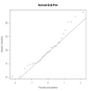
You can evaluate the normality of a variable using a Q-Q plot.
# Q-Q Plot for variable MPG
attach(mtcars)
qqnorm(mpg)
qqline(mpg)
Significant departures from the line suggest violations of normality.
You can also perform a Shapiro-Wilk test of normality with the shapiro.test(x) function, where x is a numeric vector. Additional functions for testing normality are available in nortest package.
Multivariate Normality
MANOVA assumes multivariate normality. The function mshapiro.test( ) in the mvnormtest package produces the Shapiro-Wilk test for multivariate normality. Input must be a numeric matrix.
# Test Multivariate Normality

mshapiro.test(M)
If we have p x 1 multivariate normal random vector ![]()
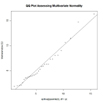
then the squared Mahalanobis distance between x and μ is going to be chi-square distributed with p degrees of freedom. We can use this fact to construct a Q-Q plot to assess multivariate normality.
# Graphical Assessment of Multivariate Normality
x <- as.matrix(mydata) # n x p numeric matrix
center <- colMeans(x) # centroid
n <- nrow(x); p <- ncol(x); cov <- cov(x);
d <-
mahalanobis(x,center,cov) # distances

qqplot(qchisq(ppoints(n),df=p),d,
  main="QQ Plot Assessing Multivariate Normality",
  ylab="Mahalanobis D2")
abline(a=0,b=1)
Homogeneity of Variances
The bartlett.test( ) function provides a parametric K-sample test of the equality of variances. The fligner.test( ) function provides a non-parametric test of the same. In the following examples y is a numeric variable and G is the grouping variable.
# Bartlett Test of Homogeneity of Variances
bartlett.test(y~G, data=mydata)

# Figner-Killeen Test of Homogeneity of Variances
fligner.test(y~G, data=mydata)
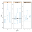
The hovPlot( ) function in the HH package provides a graphic test of homogeneity of variances based on Brown-Forsyth. In the following example, y is numeric and G is a grouping factor. Note that G must be of type factor.
# Homogeneity of Variance Plot
library(HH)
hov(y~G, data=mydata)
hovPlot(y~G,data=mydata)
Homogeneity of Covariance Matrices
MANOVA and LDF assume homogeneity of variance-covariance matrices. The assumption is usually tested with Box's M. Unfortunately the test is very sensitive to violations of normality, leading to rejection in most typical cases. Box's M is available via the boxM function in the biotools package.
To Practice
Take the Introduction to Statistics in R course to grow your statistical skills futher.


