Regression Diagnostics
An excellent review of regression diagnostics is provided in John Fox's aptly named Overview of Regression Diagnostics. Dr. Fox's car package provides advanced utilities for regression modeling.
# Assume that we are fitting a multiple linear regression
#
on the MTCARS data
library(car)
fit <- lm(mpg~disp+hp+wt+drat, data=mtcars)
This example is for exposition only. We will ignore the fact that this may not be a great way of modeling the this particular set of data!
Outliers
# Assessing Outliers
outlierTest(fit) # Bonferonni p-value for most extreme obs
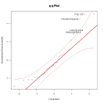
qqPlot(fit, main="QQ Plot") #qq plot for studentized resid

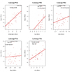
leveragePlots(fit) # leverage plots
Influential Observations
# Influential Observations
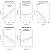
# added variable plots
av.Plots(fit)
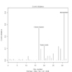
# Cook's D plot
# identify D values > 4/(n-k-1)
cutoff <- 4/((nrow(mtcars)-length(fit$coefficients)-2))
plot(fit, which=4, cook.levels=cutoff)
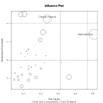
# Influence Plot

influencePlot(fit, id.method="identify", main="Influence Plot", sub="Circle size is proportial to Cook's Distance" )
Non-normality
# Normality of Residuals
# qq plot for studentized resid
qqPlot(fit, main="QQ Plot")
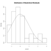
# distribution of studentized residuals
library(MASS)
sresid <- studres(fit)
hist(sresid, freq=FALSE,
   main="Distribution of Studentized Residuals")
xfit<-seq(min(sresid),max(sresid),length=40)
yfit<-dnorm(xfit)

lines(xfit, yfit)
Non-constant Error Variance
# Evaluate homoscedasticity
# non-constant error variance test
ncvTest(fit)
# plot
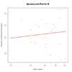
studentized residuals vs. fitted values
spreadLevelPlot(fit)
Multi-collinearity
# Evaluate Collinearity
vif(fit) # variance inflation factors
sqrt(vif(fit)) > 2 # problem?
Nonlinearity
# Evaluate Nonlinearity
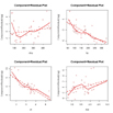
# component + residual plot
crPlots(fit)
# Ceres plots
ceresPlots(fit)
Non-independence of Errors
# Test for Autocorrelated Errors
durbinWatsonTest(fit)
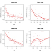
Additional Diagnostic Help
The gvlma( ) function in the gvlma package, performs a global validation of linear model assumptions as well separate evaluations of skewness, kurtosis, and heteroscedasticity.
# Global test of model assumptions
library(gvlma)
gvmodel <- gvlma(fit)

summary(gvmodel)
Going Further
If you would like to delve deeper into regression diagnostics, two books written by John Fox can help: Applied regression analysis and generalized linear models (2nd ed) and An R and S-Plus companion to applied regression.
