Discriminant Function Analysis
The MASS package contains functions for performing linear and quadratic
discriminant function analysis. Unless prior probabilities are specified, each assumes proportional prior probabilities (i.e., prior probabilities are based on sample sizes). In the examples below, lower case letters are numeric variables and upper case letters are categorical factors.
Linear Discriminant Function
# Linear Discriminant Analysis with Jacknifed Prediction

library(MASS)
fit <- lda(G ~ x1 + x2 + x3, data=mydata,
   na.action="na.omit", CV=TRUE)
fit # show results
The code above performs an LDA, using listwise deletion of missing data. CV=TRUE generates jacknifed (i.e., leave one out) predictions. The code below assesses the accuracy of the prediction.
# Assess the accuracy of the prediction
# percent correct for each category of G
ct <- table(mydata$G, fit$class)
diag(prop.table(ct, 1))
# total percent correct
sum(diag(prop.table(ct)))
lda() prints discriminant functions based on centered (not standardized) variables. The "proportion of trace" that is printed is the proportion of between-class variance that is explained by successive discriminant functions. No significance tests are produced. Refer to the section on MANOVA for such tests.
Quadratic Discriminant Function
To obtain a quadratic discriminant function use qda( ) instead of lda( ). Quadratic discriminant function does not assume homogeneity of variance-covariance matrices.
# Quadratic Discriminant Analysis with 3 groups applying
#
resubstitution prediction and equal prior probabilities.
library(MASS)
fit <- qda(G ~ x1 + x2 + x3 + x4, data=na.omit(mydata),
  prior=c(1,1,1)/3))
Note the alternate way of specifying listwise deletion of missing data. Re-subsitution (using the same data to derive the functions and evaluate their prediction accuracy) is the default method unless CV=TRUE is specified. Re-substitution will be overly optimistic.
Visualizing the Results
You can plot each observation in the space of the first 2 linear discriminant functions using the following code. Points are identified with the group ID.
# Scatter plot using the 1st two discriminant dimensions
plot(fit) # fit from lda
 click to view
The following code displays histograms and density plots for the observations in each group on the first linear discriminant dimension. There is one panel for each group and they all appear lined up on the same graph.
# Panels of histograms and overlayed density plots
# for 1st discriminant function
plot(fit, dimen=1, type="both") # fit from lda
 click to view
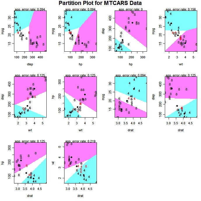
The partimat( ) function in the klaR package can display the results of a linear or quadratic classifications 2 variables at a time.
# Exploratory Graph for LDA or QDA
library(klaR)
partimat(G~x1+x2+x3,data=mydata,method="lda")
 click to view
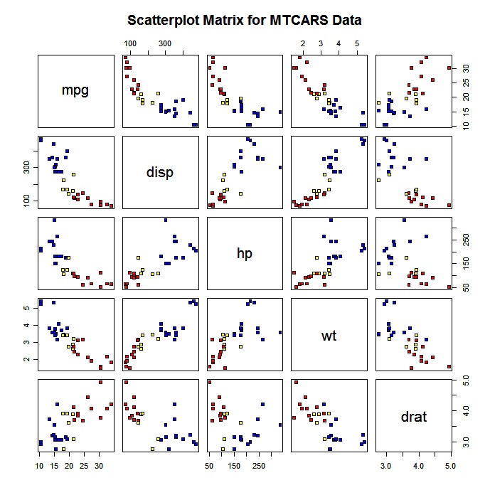
You can also produce a scatterplot matrix with color coding by group.
# Scatterplot for 3 Group Problem
pairs(mydata[c("x1","x2","x3")], main="My Title ", pch=22,
   bg=c("red", "yellow", "blue")[unclass(mydata$G)])
 click to view
Test Assumptions
See (M)ANOVA Assumptionsfor methods of evaluating multivariate normality and homogeneity of covariance matrices.
To Practice
To practice improving predictions, try the the Supervised Learning in R course