Generalized Linear Models
Generalized linear models are fit using the glm( ) function. The form of the glm function is
glm(formula , family= familytype(link=linkfunction), data=)
| Family | Default Link Function |
| binomial | (link = "logit") |
| gaussian | (link = "identity") |
| Gamma | (link = "inverse") |
| inverse.gaussian | (link = "1/mu^2") |
| poisson | (link = "log") |
| quasi | (link = "identity", variance = "constant") |
| quasibinomial | (link = "logit") |
| quasipoisson | (link = "log") |
See help(glm) for other modeling options. See help(family) for other allowable link functions for each family. Three subtypes of generalized linear models will be covered here: logistic regression, poisson regression, and survival analysis.
Logistic Regression
Logistic regression is useful when you are predicting a binary outcome from a set of continuous predictor variables. It is frequently preferred over discriminant function analysis because of its less restrictive assumptions.
# Logistic Regression
# where F is a binary factor and
# x1-x3 are continuous predictors
fit <- glm(F~x1+x2+x3,data=mydata,family=binomial())
summary(fit) # display results
confint(fit) # 95% CI for the coefficients
exp(coef(fit)) # exponentiated coefficients
exp(confint(fit)) # 95% CI for exponentiated coefficients
predict(fit, type="response") # predicted values
residuals(fit, type="deviance") # residuals
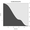
You can use anova(fit1 , fit2, test="Chisq") to compare nested models. Additionally, cdplot(F ~ x , data= mydata) will display the conditional density plot of the binary outcome F on the continuous x variable.
Poisson Regression
Poisson regression is useful when predicting an outcome variable representing counts from a set of continuous predictor variables.
# Poisson Regression
# where count is a count and
# x1-x3 are continuous predictors
fit <- glm(count ~ x1+x2+x3, data=mydata, family=poisson())
summary(fit) display results
If you have overdispersion (see if residual deviance is much larger than degrees of freedom), you may want to use quasipoisson() instead of poisson().
Survival Analysis
Survival analysis (also called event history analysis or reliability analysis) covers a set of techniques for modeling the time to an event. Data may be right censored - the event may not have occured by the end of the study or we may have incomplete information on an observation but know that up to a certain time the event had not occured (e.g. the participant dropped out of study in week 10 but was alive at that time).
While generalized linear models are typically analyzed using the glm( ) function, survival analyis is typically carried out using functions from the survival package . The survival package can handle one and two sample problems, parametric accelerated failure models, and the Cox proportional hazards model.
Data are typically entered in the format start time, stop time, and status (1=event occured, 0=event did not occur). Alternatively, the data may be in the format time to event and status (1=event occured, 0=event did not occur). A status=0 indicates that the observation is right cencored. Data are bundled into a Surv object via the Surv( ) function prior to further analyses.
survfit( ) is used to estimate a survival distribution for one or more groups.
survdiff( ) tests for differences in survival distributions between two or more groups.
coxph( ) models the hazard function on a set of predictor variables.
# Mayo Clinic Lung Cancer Data
library(survival)

# learn about the dataset
help(lung)

# create a Surv object
survobj <- with(lung, Surv(time,status))

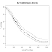
# Plot survival distribution of the total sample
# Kaplan-Meier estimator
fit0 <- survfit(survobj~1, data=lung)
summary(fit0)
plot(fit0, xlab="Survival Time in Days",
   ylab="% Surviving", yscale=100,
   main="Survival Distribution (Overall)")

# Compare the survival distributions of men and women
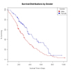
fit1 <- survfit(survobj~sex,data=lung)

# plot the survival distributions by sex
plot(fit1, xlab="Survival Time in Days",
  ylab="% Surviving", yscale=100, col=c("red","blue"),
  main="Survival Distributions by Gender")
  legend("topright", title="Gender", c("Male", "Female"),
  fill=c("red", "blue"))

# test for difference between male and female
# survival curves (logrank test)
survdiff(survobj~sex, data=lung)

# predict male survival from age and medical scores
MaleMod <- coxph(survobj~age+ph.ecog+ph.karno+pat.karno,
  data=lung, subset=sex==1)

# display results
MaleMod

# evaluate the proportional hazards assumption
cox.zph(MaleMod)
See Thomas Lumley's R news article on the survival package for more information. Other good sources include Mai Zhou's Use R Software to do Survival Analysis and Simulation and M. J. Crawley's chapter on Survival Analysis.
To Practice
Try this interactive exercise on basic logistic regression with R using age as a predictor for credit risk.


