Probability Plots
This section describes creating probability plots in R for both didactic purposes and for data analyses.
Probability Plots for Teaching and Demonstration
When I was a college professor teaching statistics, I used to have to draw normal distributions by hand. They always came out looking like bunny rabbits. What can I say?
R makes it easy to draw probability distributions and demonstrate statistical concepts. Some of the more common probability distributions available in R are given below.
| distribution | R name | distribution | R name |
| Beta | beta | Lognormal | lnorm |
| Binomial | binom | Negative Binomial | nbinom |
| Cauchy | cauchy | Normal | norm |
| Chisquare | chisq | Poisson | pois |
| Exponential | exp | Student t | t |
| F | f | Uniform | unif |
| Gamma | gamma | Tukey | tukey |
| Geometric | geom | Weibull | weib |
| Hypergeometric | hyper | Wilcoxon | wilcox |
| Logistic | logis |
For a comprehensive list, see Statistical Distributions on the R wiki. The functions available for each distribution follow this format:
| name | description |
| d name( ) | density or probability function |
| p name( ) | cumulative density function |
| q name( ) | quantile function |
| R_name_( ) | random deviates |
For example, pnorm(0) =0.5 (the area under the standard normal curve to the left of zero). qnorm(0.9) = 1.28 (1.28 is the 90th percentile of the standard normal distribution). rnorm(100) generates 100 random deviates from a standard normal distribution.
Each function has parameters specific to that distribution. For example, rnorm(100, m=50, sd=10) generates 100 random deviates from a normal distribution with mean 50 and standard deviation 10.
You can use these functions to demonstrate various aspects of probability distributions. Two common examples are given below.
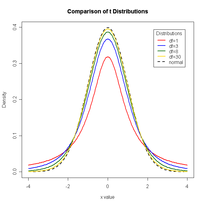
# Display the Student's t distributions with various
# degrees of freedom and compare to the normal distribution

x <- seq(-4, 4, length=100)
hx <- dnorm(x)

degf <- c(1, 3, 8, 30)
colors <- c("red", "blue", "darkgreen", "gold", "black")
labels <- c("df=1", "df=3", "df=8", "df=30", "normal")

plot(x, hx, type="l", lty=2, xlab="x value",
  ylab="Density", main="Comparison of t Distributions")

for (i in 1:4){
  lines(x, dt(x,degf[i]), lwd=2, col=colors[i])
}

legend("topright", inset=.05, title="Distributions",
  labels, lwd=2, lty=c(1, 1, 1, 1, 2), col=colors)
 click to view
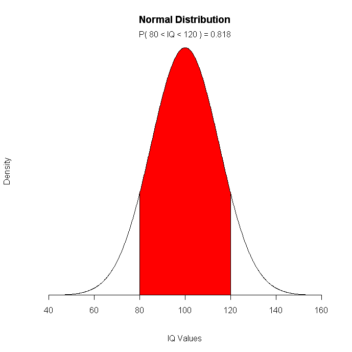
# Children's IQ scores are normally distributed with a
# mean of 100 and a standard deviation of 15. What
# proportion of children are expected to have an IQ between
# 80 and 120?

mean=100; sd=15
lb=80; ub=120

x <- seq(-4,4,length=100)*sd + mean
hx <- dnorm(x,mean,sd)

plot(x, hx, type="n", xlab="IQ Values", ylab="",
  main="Normal Distribution", axes=FALSE)

i <- x >= lb & x <= ub
lines(x, hx)
polygon(c(lb,x[i],ub), c(0,hx[i],0), col="red")

area <- pnorm(ub, mean, sd) - pnorm(lb, mean, sd)
result <- paste("P(",lb,"< IQ <",ub,") =",
  signif(area, digits=3))
mtext(result,3)
axis(1, at=seq(40, 160, 20), pos=0)
 click to view
For a comprehensive view of probability plotting in R, see Vincent Zonekynd's Probability Distributions.
Fitting Distributions
There are several methods of fitting distributions in R. Here are some options.
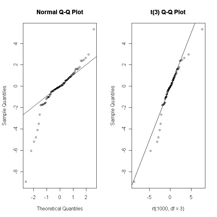
You can use the qqnorm( ) function to create a Quantile-Quantile plot evaluating the fit of sample data to the normal distribution. More generally, the qqplot( ) function creates a Quantile-Quantile plot for any theoretical distribution.
# Q-Q plots
par(mfrow=c(1,2))

# create sample data
x <- rt(100, df=3)

# normal fit
qqnorm(x);
qqline(x)

# t(3Df) fit
qqplot(rt(1000,df=3), x, main="t(3) Q-Q Plot",
  ylab="Sample Quantiles")
abline(0,1)
 click to view
The fitdistr( ) function in the MASS package provides maximum-likelihood fitting of univariate distributions. The format is fitdistr(x, densityfunction) where x is the sample data and densityfunction is one of the following: "beta", "cauchy", "chi-squared", "exponential", "f", "gamma", "geometric", "log-normal", "lognormal", "logistic", "negative binomial", "normal", "Poisson", "t" or "weibull".
# Estimate parameters assuming log-Normal distribution

# create some sample data
x <- rlnorm(100)

# estimate paramters
library(MASS)
fitdistr(x, "lognormal")
Finally R has a wide range of goodness of fit tests for evaluating if it is reasonable to assume that a random sample comes from a specified theoretical distribution. These include chi-square, Kolmogorov-Smirnov, and Anderson-Darling.
For more details on fitting distributions, see Vito Ricci's Fitting Distributions with R.
To Practice
Try this interactive course on exploratory data analysis.